Comparing YOLO 11 Retraining Strategies for Continuous Learning

I tested four YOLO 11 retraining approaches—and fine-tuning with frozen backbone layers beat full retraining while using 70% less RAM.

As part of my Jetson Posture Monitor project I wanted to compare different re-training methods for a YOLO 11 classification model. I started part 1 of the project by training a YOLO 11 classification model to detect my sitting posture. As part of adding continuous learning into the app, I wanted to test different methods of model training to decide on which method to implement in the app.

To find out, I decided to try out some different ideas of model training. I will showcase each of them, comparing the resulting model performance to evaluate the best way to implement model training as part of a continuous learning feature.

Starting point and dataset

The starting point for this test is my "reference" model I trained in part 1 of the Jetson Posture Monitor project is a YOLO 11 classification model based on the yolo11l-cls model. I trained it with ~280 images of me sitting at my desk with good and bad posture.

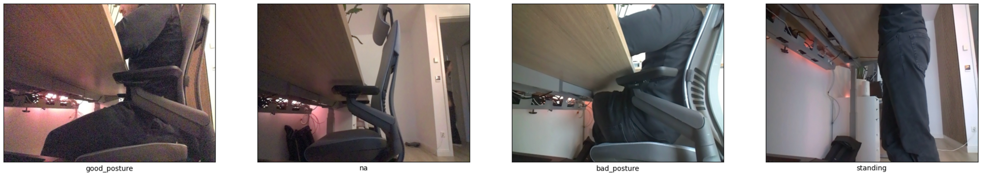
The dataset of the reference model had three classes:

• good_posture
• bad_posture
• na (me not at my desk)

For this test, I have added another ~290 images, for a total of about ~570 images just for training. I also added a fourth class standing to allow the model to also recognize me standing at my desk.

The dataset is split into the following directory structure:

.
├── dataset
│   ├── train
│   │   ├── bad_posture
│   │   ├── good_posture
│   │   ├── na
│   │   └── standing
│   ├── uncategorized
│   └── val
│       ├── bad_posture
│       ├── good_posture
│       ├── na
│       └── standing

YOLO11 Training experiments

These are the experiments I want to work through:

1. Full re-train from scratch: Start with a normal yolo11l-cls model again and re-train on the entire dataset
2. Re-train reference model with all data: Start with the already trained reference model and re-train on the entire dataset
3. Re-train reference model with new data: Start with the already trained reference model and re-train only on new data
4. Fine-tune the reference model: Start with the already trained reference model and re-train only on new data while freezing the backbone and lowering the learning rate

Throughout this post I will explain how I did the training of each. Then I will compare model performance through top1- and top5-accuracy and also by using confusion matrices.

Full re-train from scratch

For this first experiment I used the base yolo11l-cls model, and re-trained the model on the entire dataset. This completely ignores the already trained reference model. I wanted to include this test to see the difference mainly compared to re-training the reference model with the entire dataset. I was curious to see if it would make a difference if the model had already been trained on part of the dataset compared to starting fresh.

I trained the model with this Python code:

# Load YOLO base model
model = YOLO("../models/yolo11l-cls.pt")

# Train model
results = model.train(
    data='/Users/hartlden/private/jetson-posture-monitor/dataset',
    epochs=100,
    patience=30, # Stop if validation doesn't improve for multiple epochs
    imgsz=640,
    save=True,
    plots=True,
    device="mps", # Train on Apple Silicon
    name="retrain-from-scratch"
)

Training finished after 47 epochs and 67 minutes, with the best model being found at epoch 17. These are the metrics of the best model:

Re-train reference model with all data

This experiment uses the already trained reference model. It was already trained on about ~280 images, so about half of the dataset. Yet I will use the full dataset again, so the model will be trained twice on about half of the data. I wanted to include this test to see if this makes a meaningful difference, or if training only on new data makes more sense.

# Load reference model
model = YOLO("../models/reference.pt")

# Train model
results = model.train(
    data='/Users/hartlden/private/jetson-posture-monitor/dataset',
    epochs=100,
    patience=30, # Stop if validation doesn't improve for multiple epochs
    imgsz=640,
    save=True,
    plots=True,
    device="mps", # Train on Apple Silicon
    name="retrain-reference-all-data"
)

Interestingly, training finished after 31 epochs and 42 minutes on this run. The best model was instantly found at epoch 1 this time. I did not expect this, as the dataset was doubled compared to the initial training run while also adding a new fourth class.

Re-train reference model with new data

The third experiment is about re-training the reference model only on new data it has not seen before. This will serve as a good comparison to re-training on the full dataset. Could be interesting to see if there is any benefit to the model being trained on the same data multiple times.

# Load reference model
model = YOLO("../models/reference.pt")

# Train model
results = model.train(
    data='/Users/hartlden/private/jetson-posture-monitor/dataset_20251229',
    epochs=100,
    patience=30, # Stop if validation doesn't improve for multiple epochs
    imgsz=640,
    save=True,
    plots=True,
    device="mps", # Train on Apple Silicon
    name="retrain-reference-new-data"
)

This time training finished after 32 epochs and 23 minutes. The reduction in training image volume also had a significant impact on training time, as expected. The best model was found in epoch 2, so it looks like the model was able to adapt to the new class very quickly again.

Fine-tuning the reference model

The fourth and last experiment I wanted to include was to fine-tune the reference model, instead of completely training on new data. When fine-tuning, only the classification head layers within the model get trained, but backbone layers stay frozen. This significantly reduces the amount of parameters within the model which need to be re-trained. In my theory, this should significantly reduce the compute overhead for training.

I wanted to include this test because I want to implement continuous learning as part of my Jetson Posture Monitor project. The app there is running on a NVIDIA Jetson Orin Nano, so compute resources are quite limited. Reducing the compute requirements to a minimum is essential on that quite restricted platform. My goal was to see the impact freezing backbone layers had on model performance.

First, I needed to find out which layers of the model are backbone layers, and where the classification head begins.

# Get model layers to find where to freeze
model = YOLO("../models/reference.pt")
for i, (name, param) in enumerate(model.model.named_parameters()):
    print(f"{i}: {name}")

This listed every layer within the model (redacted for readability):

207: model.9.cv1.conv.weight
208: model.9.cv1.bn.weight
209: model.9.cv1.bn.bias
210: model.9.cv2.conv.weight
211: model.9.cv2.bn.weight
212: model.9.cv2.bn.bias
213: model.9.m.0.attn.qkv.conv.weight
214: model.9.m.0.attn.qkv.bn.weight
215: model.9.m.0.attn.qkv.bn.bias
216: model.9.m.0.attn.proj.conv.weight
217: model.9.m.0.attn.proj.bn.weight
218: model.9.m.0.attn.proj.bn.bias
219: model.9.m.0.attn.pe.conv.weight
220: model.9.m.0.attn.pe.bn.weight
221: model.9.m.0.attn.pe.bn.bias
222: model.9.m.0.ffn.0.conv.weight
223: model.9.m.0.ffn.0.bn.weight
224: model.9.m.0.ffn.0.bn.bias
225: model.9.m.0.ffn.1.conv.weight
226: model.9.m.0.ffn.1.bn.weight
227: model.9.m.0.ffn.1.bn.bias
228: model.9.m.1.attn.qkv.conv.weight
229: model.9.m.1.attn.qkv.bn.weight
230: model.9.m.1.attn.qkv.bn.bias
231: model.9.m.1.attn.proj.conv.weight
232: model.9.m.1.attn.proj.bn.weight
233: model.9.m.1.attn.proj.bn.bias
234: model.9.m.1.attn.pe.conv.weight
235: model.9.m.1.attn.pe.bn.weight
236: model.9.m.1.attn.pe.bn.bias
237: model.9.m.1.ffn.0.conv.weight
238: model.9.m.1.ffn.0.bn.weight
239: model.9.m.1.ffn.0.bn.bias
240: model.9.m.1.ffn.1.conv.weight
241: model.9.m.1.ffn.1.bn.weight
242: model.9.m.1.ffn.1.bn.bias
243: model.10.conv.conv.weight
244: model.10.conv.bn.weight
245: model.10.conv.bn.bias
246: model.10.linear.weight
247: model.10.linear.bias

Layer 1-10 looked very similar, but layer 11 showed a distinct break in the layer configuration, indicating the transition from backbone to classification layers. This means that the first 10 layers will stay frozen for this test.

With that knowledge, training code looks like this:

# Load reference model
model = YOLO("../models/reference.pt")

# Train model
results = model.train(
    data='/Users/hartlden/private/jetson-posture-monitor/dataset_20251229',
    epochs=100,
    patience=30, # Stop if validation doesn't improve for multiple epochs
    imgsz=640,
    save=True,
    plots=True,
    freeze=10, # Freeze the backbone layers
    device="mps", # Train on Apple Silicon
    name="retrain-finetune-new-data"
)

While I expected the second experiment to take longer for training, I expected this fine-tuning experiment to take much less time than it actually did. The training run took 92 epochs in 23 minutes, making it pretty much exactly as fast as re-training the reference model without freezing the backbone. Super interesting! The best model was only found at epoch 62.

I think training took much longer than expected because relatively speaking, the jump in dataset size was quite significant (100%), and also because a new class was introduced. I imagine that running fine-tuning more often on less significant amounts of new data would make more sense.

Evaluation and model comparison

With all the model training done, it's time to look at the results and compare them. I will keep this comparison rather simple, only looking at the top1- and top5-accuracy of each model and comparing their confusion matrices.

I used matplotlib to plot all results.

import matplotlib.pyplot as plt
from PIL import Image

%matplotlib inline

results_and_images = [
    {
        "summary": metrics_retrain_from_scratch.summary(),
        "cf": '../runs/classify/validation-retrain-from-scratch/confusion_matrix_normalized.png'
    },
    {
        "summary": metrics_retrain_reference_all_data.summary(),
        "cf": '../runs/classify/validation-retrain-reference-all-data/confusion_matrix_normalized.png'
    },
    {
        "summary": metrics_retrain_reference_new_data.summary(),
        "cf": '../runs/classify/validation-retrain-reference-new-data/confusion_matrix_normalized.png'
    },
    {
        "summary": metrics_retrain_finetune_new_data.summary(),
        "cf": '../runs/classify/validation-retrain-finetune-new-data/confusion_matrix_normalized.png'
    }
]

px = 1/plt.rcParams['figure.dpi']  # pixel in inches
fig = plt.figure(figsize=(2500*px, 2500*px))

for i, res in enumerate(results_and_images):
    ax = fig.add_subplot(2,2,i+1)
    ax.imshow(Image.open(res["cf"]))
    ax.set_xticks([])
    ax.set_yticks([])
    ax.set_xlabel(res["summary"])
plt.tight_layout()

This allows to compare all confusion matrices nicely:

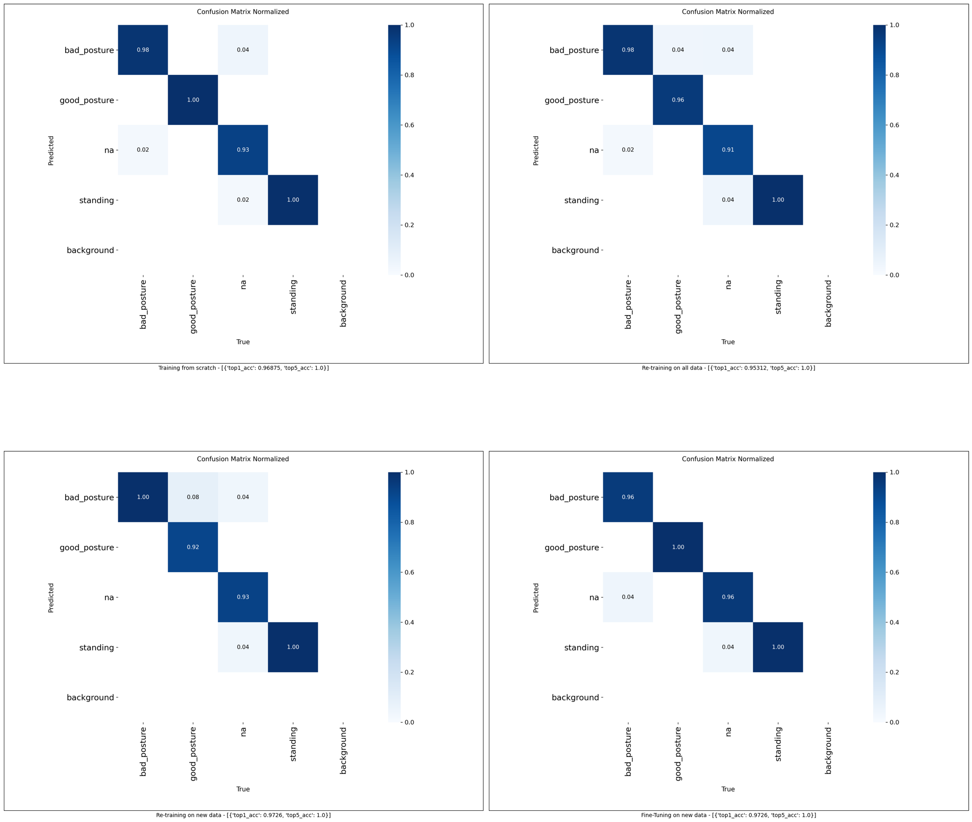
These results are not what I expected at all.

When comparing raw accuracy values, both training methods only using new data actually come out on top. When confusion matrices are also taken into account, the fine-tuning approach actually resulted in the least errors, only classifying 2 of the 73 validation images wrong.

Using validation data to compare model performances isn't ideal. Instead, using a dedicated dataset with test data, which the model has not seen during training, would be the recommended approach here. Using validation data was good enough for me in my test case however.

I absolutely expected the full train from scratch (experiment 1) to result in best performance, and fine-tuning to have the worst results. Turns out I was completely wrong on that guess 😵‍💫.

This is good news for my Jetson Posture Monitor project however. Model fine-tuning takes far less resources compared to full training. For example, experiment 3 took ~13GB of RAM and about ~40 seconds per epoch, while experiment 4 only required ~4GB of RAM and took ~12 seconds per epoch. This is on an M1 Pro Macbook Pro. This lower resource demand makes training on Jetson much more realistic and feasible, which I am very happy to hear.

Wrapping Up

It was super interesting to me to see the different approaches for model training and tuning compared and seeing their results. I absolutely had some unexpected learnings and unexpected findings which I did not expect.

You can find a Juypter Notebook with all of the code here: https://github.com/denishartl/jetson-posture-monitor/blob/main/notebooks/model-training-comparision.ipynb

Which unexpected learnings did you have when training YOLO vision models? I'd love to hear them in the comments ❤️.

If you like what you've read, I'd really appreciate it if you share this post. Thanks for reading! 🔥

Until next time! 👋

Further reading

• GitHub repo: https://github.com/denishartl/jetson-posture-monitor
• Getting started with the NVIDIA Jetson Orin Nano: https://denishartl.com/nvidia-jetson-orin-nano-first-impressions-initial-setup/
• YOLO model training documentation: https://docs.ultralytics.com/modes/train/